MSU Generalizable Notebook
Contributed by Doruk Yaldiz and Jazzmin Partridge, edited by Mark Voit
The Python code on this page demonstrates how to extend the ExpCGM implementation in the MSU Essentials Notebook to incorporate a user-defined pressure profile shape, a user-defined gravitational potential, and non-thermal atmospheric support energy. To copy and paste a cell into your own Python notebook, move your cursor to the upper right corner of the cell and click on the clipboard icon that appears.
Before executing the cells that follow, import these items:
import numpy as np
import scipy.integrate as integrate
import matplotlib.pyplot as plt
from ipywidgets import interact, FloatSlider
User-Defined Pressure Profiles
To implement a pressure profile that is not a simple power law, an ExpCGM user needs to specify the pressure profile’s shape by supplying a shape function $\alpha(x)$ that depends on a dimensionless radius $x$.
We will demonstrate how to do that by implementing the generalized NFW profile discussed on the Pressure Profiles page. Its shape function is \(\alpha(x) = - \alpha_\mathrm{in} - (\alpha_\mathrm{out} - \alpha_\mathrm{in} ) \left[ \frac{(x/x_\alpha)^{\alpha_\mathrm{tr}}} {1+(x/x_\alpha)^{\alpha_\mathrm{tr}}} \right]\) The pressure profile’s power-law slope therefore approaches $\alpha_\mathrm{in}$ at small radii and steepens to $\alpha_\mathrm{out}$ at large radii. The transition in slope happens near the radius $x_\alpha$, and the $\alpha_\mathrm{tr}$ parameter governs the sharpness of the transition.
The following cell defines a generalized NFW shape function with the parameter set $\alpha_\mathrm{in} = 1.0$, $\alpha_\mathrm{out} = 3.4$, $\alpha_\mathrm{tr} = 1.0$, and $x_\alpha = 2.16$. Users can customize the pressure profile either by adjusting these parameters or by defining $\alpha (x)$ to be a different function:
# Generalized NFW pressure profile function with default parameters

def alpha(x):
    alpha_in = 1.0
    alpha_out = 3.4
    alpha_tr = 1.0
    x_alpha = 2.16
    y = ( x / x_alpha )**alpha_tr
    return alpha_in + (alpha_out - alpha_in) * y / ( 1 + y)
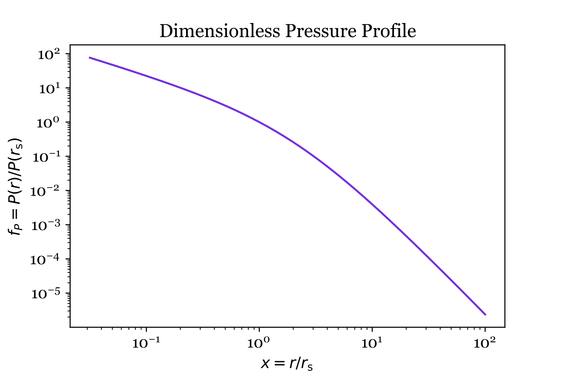
A numerical integration is needed to determine the dimensionless pressure profile function $f_P(x)$ because $\alpha(x)$ is not constant. Executing the next cell defines a function that integrates $\alpha (x) / x$ over $dx$ to obtain \(f_P(r) = \exp \left[ -\int_1^{r/r_\mathrm{s}} \frac {\alpha(x)} {x} dx \right]\) Note that the dimensionless pressure profile is normalized to unity at $r = r_\mathrm{s}$.
# Numerical integration of shape function to obtain a dimensionless pressure profile

def integrandf_P(t):
    return alpha(t) / t

def f_P(x):
    resultf_P, _ = integrate.quad(integrandf_P, 1, x, limit=50)
    return np.exp(-resultf_P)
To check the result, executing the next cell makes a plot showing $f_P(x)$:
# Makes a plot of the dimensionless pressure profile

# Specify the domain of x and determine f_P(x)
x_values = np.logspace(-1.5, 2, 50)
y_values = [f_P(x) for x in x_values]

# Choose a font
gfont = {'fontname':'georgia'}
plt.rcParams['font.family'] = 'georgia'
plt.rcParams['font.size'] = 12

plt.plot(x_values, y_values, color='blueviolet')
plt.xscale('log')
plt.yscale('log')
plt.xlabel(r'$x = r / r_\mathrm{s}$', fontsize=12)
plt.ylabel(r'$f_P = P(r)/P(r_\mathrm{s})', fontsize=12)

plt.title('Dimensionless Pressure Profile', **gfont)
plt.show()
In the ExpCGM framework, a pressure profile’s normalization depends on the atmosphere’s mean specific energy ($\varepsilon_\mathrm{CGM}$). The normalization factor for this pressure profile is \(P_0 = P(r_\mathrm{s}) = \frac {M_\mathrm{CGM} v_\varphi^2} {4 \pi r_\mathrm{s}^3} \frac {1} {I(x_\mathrm{CGM})}\) The function $I(x)$ is an integral proportional to the cumulative enclosed gas-mass profile, and $x_\mathrm{CGM}$ is a dimensionless radius that solves $\varepsilon_\mathrm{CGM} = v_\varphi^2 F(x_{\rm CGM})$, as explained on the Essentials page.
User-Defined Potential Wells
The default choice for a halo potential well in ExpCGM is an NFW potential well, expressed in terms of the dimensionless functions defined in the following cell. They are normalized so that the maximum circular velocity is unity:
# NFW halo potential well functions

A_NFW = 4.625      # Normalization constant for the NFW potential well

def phi_NFW(x):
    return A_NFW * ( 1 - np.log(1+x)/x )

def vc2_NFW(x):
    return A_NFW * ( np.log(1+x) / x - 1 / (1+x) )
Multiplying each of these functions by $v_\varphi^2$, the square of the halo’s maximum circular velocity, makes them dimensional quantities. You may also choose to replace the NFW potential functions defined here with a user-defined potential well.
To illustrate how to customize an ExpCGM atmosphere model’s potential well, we will extend the NFW halo model by adding a central galaxy potential having a maximum circular velocity $v_\mathrm{H} = f_\mathrm{H} v_\varphi$, where $f_\mathrm{H}$ is an adjustable model parameter. To represent the central galaxy’s potential well, we will use a Hernquist model with a scale radius $r_\mathrm{H} = x_\mathrm{H} r_\mathrm{s}$: \(\varphi_\mathrm{H} = 4 v_\mathrm{H}^2 \left( 1 + \frac {r_\mathrm{H}} {r + r_\mathrm{H}} \right)\)
The dimensionless functions in this cell are defined so that they give the appropriate dimensional quantities when multiplied by $v_\varphi^2$ or $v_\varphi$:
def phi_gal(x,x_H,f_H):
    return 4 * f_H**2 * (1 - x_H / (x + x_H) )

def vc2_gal(x,x_H,f_H):
    return 4 * f_H**2 * x_H * x / (x + x_H)**2

def phi(x,x_H,f_H):
    return phi_NFW(x) + phi_gal(x,x_H,f_H)

def vc2(x,x_H,f_H):
    return vc2_NFW(x) + vc2_gal(x,x_H,f_H)

def vc(x,x_H,f_H):
    return np.sqrt(vc2(x,x_H,f_H))
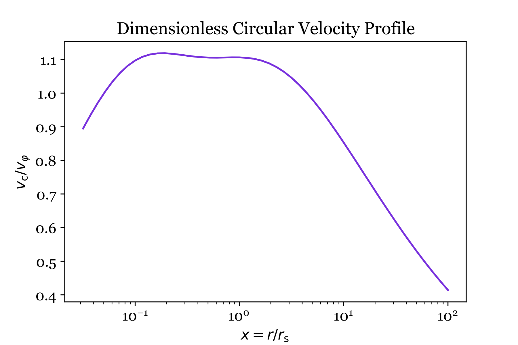
To check the result, the next cell makes a plot showing $v_\mathrm{c}(x)/v_\varphi$ for $x_H = 0.1$ and $f_H = 1.0$:
# Set the default parameters of the Hernquist model
x_H = 0.1
f_H = 1.0

# Specify the domain of x and determine v_c
x_values = np.logspace(-1.5, 2, 50)
vc_values = [vc(x,x_H,f_H) for x in x_values]

# Choose a font
gfont = {'fontname':'georgia'}
plt.rcParams['font.family'] = 'georgia'
plt.rcParams['font.size'] = 12

# Make the plot
plt.plot(x_values, vc_values, color='blueviolet')
plt.xscale('log')
plt.yscale('linear')
plt.xlabel(r'$x = r / r_\mathrm{s}$', fontsize=12)
plt.ylabel(r'$v_\mathrm{c} / v_\varphi$', fontsize=12)

plt.title('Dimensionless Circular Velocity Profile', **gfont)
plt.show()
Normalization of Circular Velocity Profile
A circular velocity profile’s normalization factor $v_\varphi$ depends on the total halo mass $M_\mathrm{halo}$ within a bounding radius $r_\mathrm{halo}$. The usual procedure for calculating it defines the halo’s radius so that the mean matter density within $r_\mathrm{halo}$ is $\Delta_\mathrm{halo}$ times the universe’s critical density at the halo’s redshift $z$. Then the circular velocity at $r_\mathrm{halo}$ is \(v_\mathrm{c}(r_\mathrm{halo}) = \left( \frac {\Delta_\mathrm{halo}} {2} \right)^{1/6} \left[ G M_\mathrm{halo} H(z) \right]^{1/3}\) The following cell therefore defines two functions:
- vhalo_kms returns $v_\mathrm{halo}$ in units of kilometers per second when given $M_\mathrm{halo}$ in units of solar mass along with $z$ and $\Delta_\mathrm{halo}$
- v_phi_NFW returns an NFW halo’s normalization factor $v_\varphi$ when given $v_\mathrm{halo}$ and the halo concentration parameter $c_\mathrm{halo} = r_\mathrm{halo} / r_\mathrm{s}$
# Returns the circular velocity (in km/s) at the radius r_halo containing the mass M_halo (in MSun)

def vhalo_kms(M_halo,z,Delta):

  # Specify some constants
  G = 6.67e-8     # gravitational constant in cgs units
  H0 = 1./4.4e17  # current Hubble constant in inverse seconds
  MSun = 2.e33    # solar mass in grams
  Omat = 0.3      # cosmological matter density parameter

  # Determine H(z)
  Hz = H0 * np.sqrt( Omat * (1+z)**3 + (1 - Omat) )

  # Convert M_halo to grams
  M_halo_grams = M_halo * MSun

  # Determine v_c  at r_halo
  vc_rhalo_cgs = ( Delta / 2 )**(1/6) * ( G * M_halo_grams * Hz )**(1/3)

  # Return vc(rhalo) in km/s
  return vc_rhalo_cgs / 1e5


# Returns the normalization factor v_phi for an NFW halo in the same units as v_halo

def v_phi_NFW(v_halo,c_halo):
  return v_halo / np.sqrt( vc2_NFW(c_halo) )
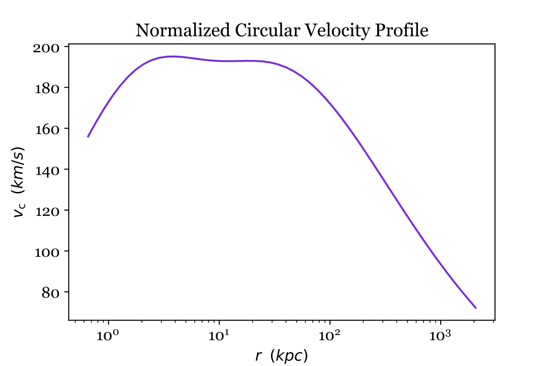
Once those functions are defined, executing the next cell makes a plot showing a properly normalized circular velocity profile:
# Set the parameters of the NFW halo model
M_halo = 1e12
z_halo = 0.0
c_halo = 10
Delta_halo = 200

# Determine v_phi for the NFW profile
v_phi = v_phi_NFW(vhalo_kms(M_halo,z_halo,Delta_halo),c_halo)

# Determine r_halo for the NFW model
G = 6.67e-8
cm_per_kpc = 3.08e21
g_per_MSun = 2e33
rhalo_cm = G * M_halo * g_per_MSun / (vhalo_kms(M_halo,z_halo,Delta_halo) * 1e5)**2
rhalo_kpc = rhalo_cm / cm_per_kpc

# Specify the domain of x and determine r in kpc and v_c in km/s
x_values = np.logspace(-1.5, 2, 50)
r_values = [x * rhalo_kpc / c_halo for x in x_values]
vc_values = [v_phi * vc(x,x_H,f_H) for x in x_values]

# Choose a font
gfont = {'fontname':'georgia'}
plt.rcParams['font.family'] = 'georgia'
plt.rcParams['font.size'] = 12

# Make the plot
plt.plot(r_values, vc_values, color='blueviolet')
plt.xscale('log')
plt.yscale('linear')
plt.xlabel(r'$r$  (kpc)', fontsize=12)
plt.ylabel(r'$v_\mathrm{c} \; \;  (km/s)$', fontsize=12)

plt.title('Normalized Circular Velocity Profile', **gfont)
plt.show()
Non-thermal Support Energy
Non-thermal forms of atmospheric support energy can be accounted for with the $f_\mathrm{th}$ and $f_\varphi$ parameters defined on the Essentials page. Each parameter can be a user-defined function of radius that is included in the integrals for the cumulative mass and energy integrals.
Here we define functions that simply set those parameters equal to unity and include a function for $\alpha_\mathrm{eff}$ that becomes important when $f_\mathrm{th}$ depends on radius:
# Assume all of the atmospheric support energy is thermal
def fth(x):
  fth_unity = 1
  return fth_unity

# Assume actual gravitational acceleration is not modified
def fphi(x):
  fphi_unity = 1
  return fphi_unity

# Effective shape function accounting for gradients in f_th
def alpha_eff(x):
  dx = 0.01 * x
  dfth = fth(x + dx/2) - fth(x - dx/2)
  return alpha(x) + x / fth(x) * dfth / dx
Generalized Cumulative Mass and Energy Integrals
When the pressure profile’s shape function depends on radius, the ExpCGM integrals for cumulative mass and energy need to have $\alpha(x)$ inside them, unlike in the MSU Essentials Notebook. This cell defines functions compute those integrals based on a user-defined shape function:
# Functions performing mass and energy integrals for a radius-dependent shape function

# Set a lower limit on x=r/r_s for numerical integrations
eps = 10**(-4)

# Integrate to obtain cumulative mass profile
def integrandI(t,x_H,f_H):
    return alpha_eff(t) * f_P(t) * t**2 / ( fth(t) * fphi(t) * vc2(t,x_H,f_H) )
def I(x,x_H,f_H):
    resultI, _ = integrate.quad(integrandI, eps, x, limit=50)
    return resultI

# Integrate to obtain cumulative gravitational energy profile
def integrandJphi(t,x_H,f_H):
    return alpha_eff(t) * f_P(t) * phi(t,x_H,f_H) * t**2 / ( fth(t) * fphi(t) * vc2(t,x_H,f_H) )
def Jphi(t):
    resultJphi, _ = integrate.quad(integrandJphi, eps, x, limit=50)
    return resultJphi

# Integrate to obtain cumulative thermal energy profile
def integrandJth(t):
    return f_P(t) * t**2
def Jth(x):
    resultJth, _ = integrate.quad(integrandJth, eps, x, limit=50)
    return 3 / 2 * resultJth

# Integrate to obtain cumulative non-thermal energy profile for effective adiabatic index of 5/3
def integrandJnt(t):
    gamma_nt = 5/3
    return ( 1 - fth(t) ) / fth(t) * f_P(t) * t**2 / ( gamma_nt - 1 )
def Jnt(x):
    resultJth, _ = integrate.quad(integrandJth, eps, x, limit=50)
    return 3 / 2 * resultJth

def F(x):
    return (Jphi(x) + Jth(x) + Jnt(x)) / I(x)
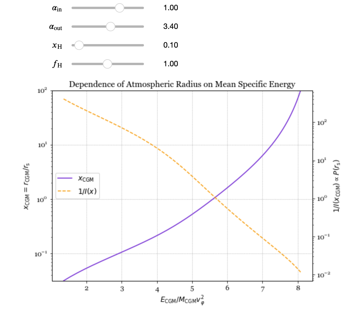
Interactive Plot of $r_\mathrm{CGM} (\varepsilon_\mathrm{CGM})$
# Code to make an interactive epsCGM-xCGM plot (assuming fth = fphi = 1)

# Generalized NFW pressure profile function adjustable parameters (alpha_in, alpha_out)

def alpha_gNFW(x,alpha_in,alpha_out):
    alpha_tr = 1.0
    x_alpha = 2.163
    y = ( x / x_alpha )**alpha_tr
    return alpha_in + (alpha_out - alpha_in) * y / ( 1 + y)

# Numerical integration of shape function to obtain a dimensionless pressure profile

def integrandf_P(t,alpha_in,alpha_out):
    return alpha_gNFW(t,alpha_in,alpha_out) / t

def f_P(x,alpha_in,alpha_out):
    resultf_P, _ = integrate.quad(integrandf_P, 1, x, args=(alpha_in,alpha_out,),
                                  limit=50)
    return np.exp(-resultf_P)

# Set a lower limit on x=r/r_s for numerical integrations
eps = 10**(-4)

# Integral for cumulative mass profile
def integrandI(t,alpha_in,alpha_out,x_H,f_H):
    return alpha_gNFW(t,alpha_in,alpha_out) * f_P(t,alpha_in,alpha_out) * t**2 / vc2(t,x_H,f_H)
def I(x,alpha_in,alpha_out,x_H,f_H):
    resultI, _ = integrate.quad(integrandI, eps, x, args=(alpha_in,alpha_out,x_H,f_H,),
                                limit=50)
    return resultI

# Integral for cumulative gravitational energy profile
def integrandJphi(t,alpha_in,alpha_out,x_H,f_H):
    return alpha_gNFW(t,alpha_in,alpha_out) * f_P(t,alpha_in,alpha_out) * phi(t,x_H,f_H) * t**2 / vc2(t,x_H,f_H)
def Jphi(x,alpha_in,alpha_out,x_H,f_H):
    resultJphi, _ = integrate.quad(integrandJphi, eps, x, args=(alpha_in,alpha_out,x_H,f_H,), limit=50)
    return resultJphi

# Integrate to obtain cumulative thermal energy profile
def integrandJth(t,alpha_in,alpha_out):
    return f_P(t,alpha_in,alpha_out) * t**2
def Jth(x,alpha_in,alpha_out):
    resultJth, _ = integrate.quad(integrandJth, eps, x, args=(alpha_in,alpha_out,), limit=50)
    return 3 / 2 * resultJth

def F(x,alpha_in,alpha_out,x_H,f_H):
    return (Jphi(x,alpha_in,alpha_out,x_H,f_H) + Jth(x,alpha_in,alpha_out)) / I(x,alpha_in,alpha_out,x_H,f_H)

# Function update_gNFW for updating the plot

def update_gNFW(alpha_in=1.0,alpha_out=3.4,x_H=0.1,f_H=1.0):

    # To prepare the plot, specify a range of x and determine the range of F(x) and 1/I(x)
    x_values = np.logspace(-1.5, 2, 50)
    y1_values = [F(x,alpha_in,alpha_out,x_H,f_H) for x in x_values]
    y2_values = [1/I(x,alpha_in,alpha_out,x_H,f_H) for x in x_values]

    # Choose a font
    gfont = {'fontname':'georgia'}
    plt.rcParams['font.family'] = 'georgia'
    plt.rcParams['font.size'] = 12

    # Specify a figure size
    fig, ax1 = plt.subplots(figsize=(8, 6))

    # Plot x_CGM as a function of F(x_CGM) using a solid blue-violet line
    ax1.plot(y1_values, x_values, color='blueviolet', label='$x_{\mathrm{CGM}}$')
    ax1.set_xscale('linear')
    ax1.set_yscale('log')
    ax1.set_xlabel(r'$E_\mathrm{CGM} / M_\mathrm{CGM} v_{\varphi}^2$', fontsize=12)
    ax1.set_ylabel(r'$x_\mathrm{CGM} = r_\mathrm{CGM} / r_\mathrm{s}$', fontsize=12)
    ax1.set_ylim(10**-1.5, 10**2)
    ax1.grid(True, linestyle='--', linewidth=0.5)

    # Plot 1/I(x_CGM) as a function of F(x_CGM) using a dashed orange line
    ax2 = ax1.twinx()
    ax2.plot(y1_values, y2_values, color='orange', linestyle='--', label='$1/I(x)$')
    ax2.set_ylabel('$1/I(x_\mathrm{CGM}) \propto P(r_\mathrm{s})$', fontsize=12)
    ax2.set_yscale('log')

    # Add a legend
    lines_1, labels_1 = ax1.get_legend_handles_labels()
    lines_2, labels_2 = ax2.get_legend_handles_labels()
    ax1.legend(lines_1 + lines_2, labels_1 + labels_2, loc='center left')

    # Add a title and show the plot
    plt.title('Dependence of Atmospheric Radius on Mean Specific Energy', **gfont)
    plt.show()
#    plt.savefig('epsCGM_xCGM_generalized.pdf')

# Make the interactive plot
#   continuous_update=True allows the graph to update while slider is moved
#   continuous_update=False updates the graph after the slider stops moving

alpha_in_slider = FloatSlider(description=r'$\alpha_\mathrm{in}$', min=0.0, max=1.5, step=0.01, value=1.0,
                           continuous_update=False)
alpha_out_slider = FloatSlider(description=r'$\alpha_\mathrm{out}$', min=1.5, max=5.0, step=0.01, value=3.4,
                           continuous_update=False)
x_H_slider = FloatSlider(description=r'$x_\mathrm{H}$', min=0.05, max=0.5, step=0.01, value=0.1,
                           continuous_update=False)
f_H_slider = FloatSlider(description=r'$f_\mathrm{H}$', min=0.0, max=2.0, step=0.01, value=1.0,
                           continuous_update=False)
interact(update_gNFW, alpha_in=alpha_in_slider, alpha_out=alpha_out_slider,
                         x_H=x_H_slider, f_H=f_H_slider);
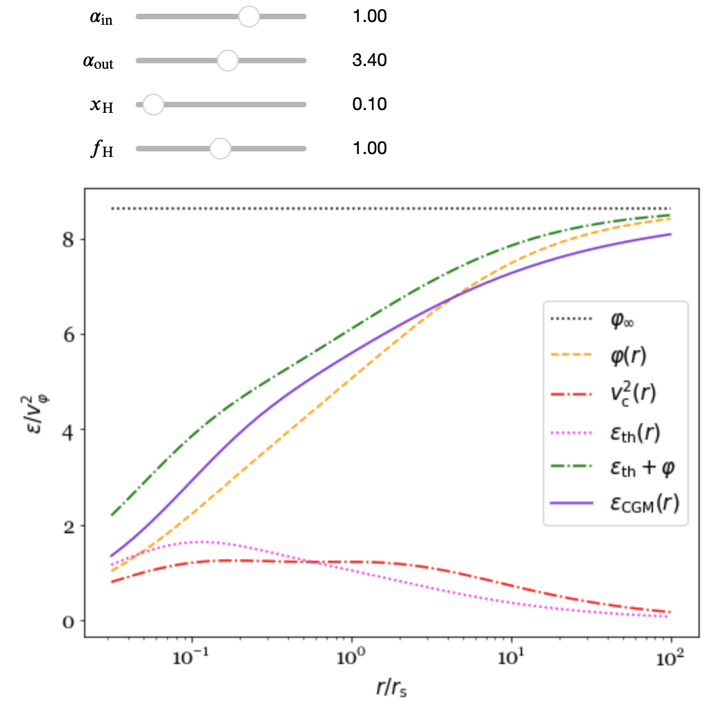
Interactive Plot Showing Specific Energy Profiles
def update_epsilon(alpha_in=1.0,alpha_out=3.4,x_H=0.1,f_H=1.0):

    # To prepare the plot, specify a range of x and determine the range of F(x)
    x_values = np.logspace(-1.5, 2, 50)
    f_values = [F(x,alpha_in,alpha_out,x_H,f_H) for x in x_values]

    # Determine individual specific energy profiles
    phi_values = [phi(x,x_H,f_H) for x in x_values]
    vc2_values = [vc2(x,x_H,f_H) for x in x_values]
    eps_th_values = [1.5 * vc2(x,x_H,f_H) / alpha_gNFW(x,alpha_in,alpha_out) \
                    for x in x_values]
    eps_values = [phi(x,x_H,f_H) + 1.5 * vc2(x,x_H,f_H) / alpha_gNFW(x,alpha_in,alpha_out) \
                    for x in x_values]

    # Determine the potential at infinity, for reference
    x_big = 1e6
    phi_infty = phi(x_big,x_H,f_H)
    phi_infty_values = [phi_infty for x in x_values]

    # Specify plot characteristics
    gfont = {'fontname':'georgia'}
    plt.rcParams['font.family'] = 'georgia'
    plt.rcParams['font.size'] = 15
    plt.figure(figsize=(8, 6))
    plt.xscale('log')
    plt.yscale('linear')
    plt.xlabel(r'$r / r_\mathrm{s}$', fontsize=15)
    plt.ylabel(r'$\varepsilon / v_\varphi^2$', fontsize=15)

    # Plot the profiles
    plt.plot(x_values, phi_infty_values, color='black', linestyle=':', \
                     label=r'$\varphi_\infty$')
    plt.plot(x_values, phi_values, color='orange', linestyle='--', \
                     label=r'$\varphi (r)$')
    plt.plot(x_values, vc2_values, color='red', linestyle='-.', \
                     label=r'$v_\mathrm{c}^2 (r)$')
    plt.plot(x_values, eps_th_values, color='magenta', linestyle=':', \
                     label=r'$\varepsilon_\mathrm{th} (r)$')
    plt.plot(x_values, eps_values, color='green', linestyle='-.', \
                     label=r'$\varepsilon_\mathrm{th} + \varphi$')
    plt.plot(x_values, f_values, color='blueviolet', linestyle='-', \
                     label=r'$\varepsilon_\mathrm{CGM}(r)$')

    # Add a legend
    plt.legend(loc='center right')

    # Show the plot
    plt.show()

# Specify sliders for adjustable parameters and make the plot interactive
alpha_in_slider = FloatSlider(description=r'$\alpha_\mathrm{in}$', min=0.0, max=1.5, \
                         step=0.01, value=1.0, continuous_update=False)
alpha_out_slider = FloatSlider(description=r'$\alpha_\mathrm{out}$', min=1.5, max=5.0, \
                         step=0.01, value=3.4, continuous_update=False)
x_H_slider = FloatSlider(description=r'$x_\mathrm{H}$', min=0.05, max=0.5, \
                         step=0.01, value=0.1, continuous_update=False)
f_H_slider = FloatSlider(description=r'$f_\mathrm{H}$', min=0.0, max=2.0, \
                         step=0.01, value=1.0, continuous_update=False)

interact(update_epsilon, alpha_in=alpha_in_slider, alpha_out=alpha_out_slider, \
                         x_H=x_H_slider, f_H=f_H_slider);