MSU Essentials Notebook

Contributed by Doruk Yaldiz and Jazzmin Partridge, edited by Mark Voit

The Python notebook cells on this page present an implementation of the ExpCGM framework that relates a galactic atmosphere’s radius to its mean specific energy, based on simple assumptions about the atmosphere’s pressure profile and gravitational potential well. To copy and paste a cell into your own notebook, move your cursor to the upper right corner of the cell and click on the clipboard icon that appears.

Before executing the rest of the cells, you will want to import a few items:

import numpy as np
import scipy.integrate as integrate
import matplotlib.pyplot as plt
from ipywidgets import interact, FloatSlider

Power‑Law Atmosphere in an NFW Potential

All ExpCGM atmosphere models begin with a shape function, defined on the Essentials page, that specifies the shape of a galactic atmosphere’s radial pressure profile: \(\alpha(r) = -\frac{d\ln P}{d\ln r}\) Here we will use the simplest shape function: a constant value of $\alpha$ resulting in a power-law pressure profile. The MSU Generalizable Notebook demonstrates how to implement shape functions that depend on radius.

This basic ExpCGM model also assumes an NFW gravitational potential: \(\varphi_{\rm NFW} (x) = A_{\rm NFW} \, v_\varphi^2 \, \left[ 1 - \frac {\ln (1+x)}{x} \right]\) Here, $x = r/r_{\rm s}$ represents radius in units of the NFW profile’s scale radius $r_{\rm s}$, and $A_{\rm NFW} = 4.625$ is a normalization constant that makes the profile’s maximum circular velocity (at $x = 2.163$) equal to $v_\varphi$. Note that we have chosen the potential’s zero point to be at $r = 0$.

Pressure Profile and Circular Velocity Profile

In general, a dimensionless pressure-profile function $f_P$ is obtained by integrating the shape function $\alpha (x)$ over $\ln x$. However, no integration is necessary for constant $\alpha$. We can simply define the pressure-profile function to be \(f_P(r) = \left(\frac{r}{r_0}\right)^{-\alpha}\) where $r_0$ is the radius at which $f_P$ is normalized to unity.

The NFW potential function is given above, but we will also be using a circular velocity profile function obtained by differentating $\varphi(x)$ with repect to $x$ and then multiplying the result by $x$: \(v_c^2(x) = A_{\rm NFW}\, v_\varphi^2\, \left[ \frac{\ln(1+x)}{x} - \frac{1}{1+x} \right]\)

This cell defines three functions determining how those profiles depend on $x = r / r_{\rm s}$:

# Dimensionless pressure profile f_P is a power law equal to unity at r = r_s:

alpha = 1.5       # default power-law slope for the pressure profile

def f_P(x,alpha):        
    return x**(-alpha)

# Dimensionless NFW potential well is normalized so that max(vc) is unity

A_NFW = 4.625     # NFW profile normalization constant 

def phi(x):
    return A_NFW * ( 1 - np.log(1 + x) / x ) 

def vc2(x):
    return A_NFW * ( np.log(1 + x) / x - 1 / (1 + x) )

Cumulative Mass and Energy Integrals

The Essentials page explains how ExpCGM determines a galactic atmosphere’s total specific energy $\varepsilon_{\rm CGM} = E_{\rm CGM} / M_{\rm CGM}$ by way of several dimensionless integrals:

\(I(x) = v_\varphi^2 \int_0^x \frac{\alpha(x)f_P(x)}{v_c^2(x)}x^2\,dx \; \; \; \; \text{(cumulative gas mass)}\) \(J_\varphi(x) = \int_0^x \frac{\alpha(x)f_P(x)\varphi(x)}{v_c^2(x)}x^2\,dx \; \; \; \; \text{(cumulative gravitational energy)}\) \(J_{\rm th}(x) = \frac{3}{2} \int_0^x f_P(x)\,x^2\,dx \; \; \; \; \text{(cumulative thermal energy)}\)

In this example, we are modeling an atmosphere supported entirely by thermal energy $(f_{\rm th} = 1)$ and so we do not need an integral that calculates cumulative non-thermal energy.

The total specific energy of this model atmosphere is \(\varepsilon_{\rm CGM} = \frac{E_{\rm CGM}}{M_{\rm CGM}} = v_\varphi^2\, F\left(\frac{r_{\rm CGM}}{r_0}\right)\) where $F(x)$ is a dimensionless profile function tracking the atmosphere’s mean specific energy within $x$: \(F(x) = \frac{J_\varphi(x) + J_{\rm th}(x)}{I(x)}\)

This cell defines functions that compute the necessary dimensionless mass and energy integrals:

# For each integral we first define a function providing the integrand, then do the integration

# Set a lower limit on x=r/r_s for numerical integrations
eps = 10**(-4)    

# Cumulative gas mass profile
def integrandI(t,alpha): 
    return f_P(t,alpha) * t**2 / vc2(t)
def I(x,alpha):        
    resultI, _ = integrate.quad(integrandI, eps, x, args=(alpha,), limit=50)
    return alpha * resultI

# Cumulative gravitational energy profile
def integrandJphi(t,alpha):
    return f_P(t,alpha) * phi(t) / vc2(t) * t**2
def Jphi(x,alpha):
    resultJphi, _ = integrate.quad(integrandJphi, eps, x, args=(alpha,), limit=50)
    return alpha * resultJphi

# Cumulative thermal energy profile
def integrandJth(t,alpha):
    return f_P(t,alpha) * t**2
def Jth(x,alpha):
    resultJth, _ = integrate.quad(integrandJth, eps, x, args=(alpha,), limit=50)
    return 3 / 2 * resultJth

# Mean specific energy profile
def F(x,alpha):
    return (Jphi(x,alpha) + Jth(x,alpha)) / I(x,alpha)

Plotting the Dependence of $r_{\rm CGM}$ on $\varepsilon_{\rm CGM}$

We now have the tools needed to reproduce the plot on the Essentials page, showing how $x_{\rm CGM} = r_\mathrm{CGM} / r_{\rm s}$ depends on $\varepsilon_{\rm CGM}/v_\varphi^2$ for $\alpha = 1.5$. The procedure first computes the dependence of $F(x_{\rm CGM})$ on $x_{\rm CGM}$. Then it inverts that dependence to obtain the desired plot.

The plot also shows how the pressure-profile normalization factor $P_0$ declines as $\varepsilon_{\rm CGM}$ rises and the atmosphere expands. Note that $P_0$ is the pressure at $r = r_{\rm s}$ in this example. It is inversely proportional to $I(x_{\rm CGM})$, and the normalization factor is given on the Essentials page.

# To prepare the plot, specify a range of x and determine the range of F(x) and 1/I(x)
x_values = np.logspace(-1.5, 2, 50)
y1_values = [F(x,alpha) for x in x_values]
y2_values = [1/I(x,alpha) for x in x_values]

# Choose a font
gfont = {'fontname':'georgia'}
plt.rcParams['font.family'] = 'georgia' 
plt.rcParams['font.size'] = 12 

# Specify a figure size
fig, ax1 = plt.subplots(figsize=(8, 6))

# Plot x_CGM as a function of F(x_CGM) using a solid blue-violet line
ax1.plot(y1_values, x_values, color='blueviolet', label='$x_{\mathrm{CGM}}$')
ax1.set_xscale('linear')
ax1.set_yscale('log')
ax1.set_xlabel(r'$E_\mathrm{CGM} / M_\mathrm{CGM} v_{\varphi}^2$', fontsize=12)
ax1.set_ylabel(r'$x_\mathrm{CGM} = r_\mathrm{CGM} / r_\mathrm{s}$', fontsize=12)
ax1.set_ylim(10**-1.5, 10**2)
ax1.grid(True, linestyle='--', linewidth=0.5)

# Plot 1/I(x_CGM) as a function of F(x_CGM) using a dashed orange line
ax2 = ax1.twinx()
ax2.plot(y1_values, y2_values, color='orange', linestyle='--', label='$1/I(x)$')
ax2.set_ylabel('$1/I(x_\mathrm{CGM})$', fontsize=12)
ax2.set_yscale('log')

# Add a legend
lines_1, labels_1 = ax1.get_legend_handles_labels()
lines_2, labels_2 = ax2.get_legend_handles_labels()
ax1.legend(lines_1 + lines_2, labels_1 + labels_2, loc='center left')

# Add a title and show the plot
plt.title('Dependence of Atmospheric Radius on Mean Specific Energy', **gfont)
plt.show()

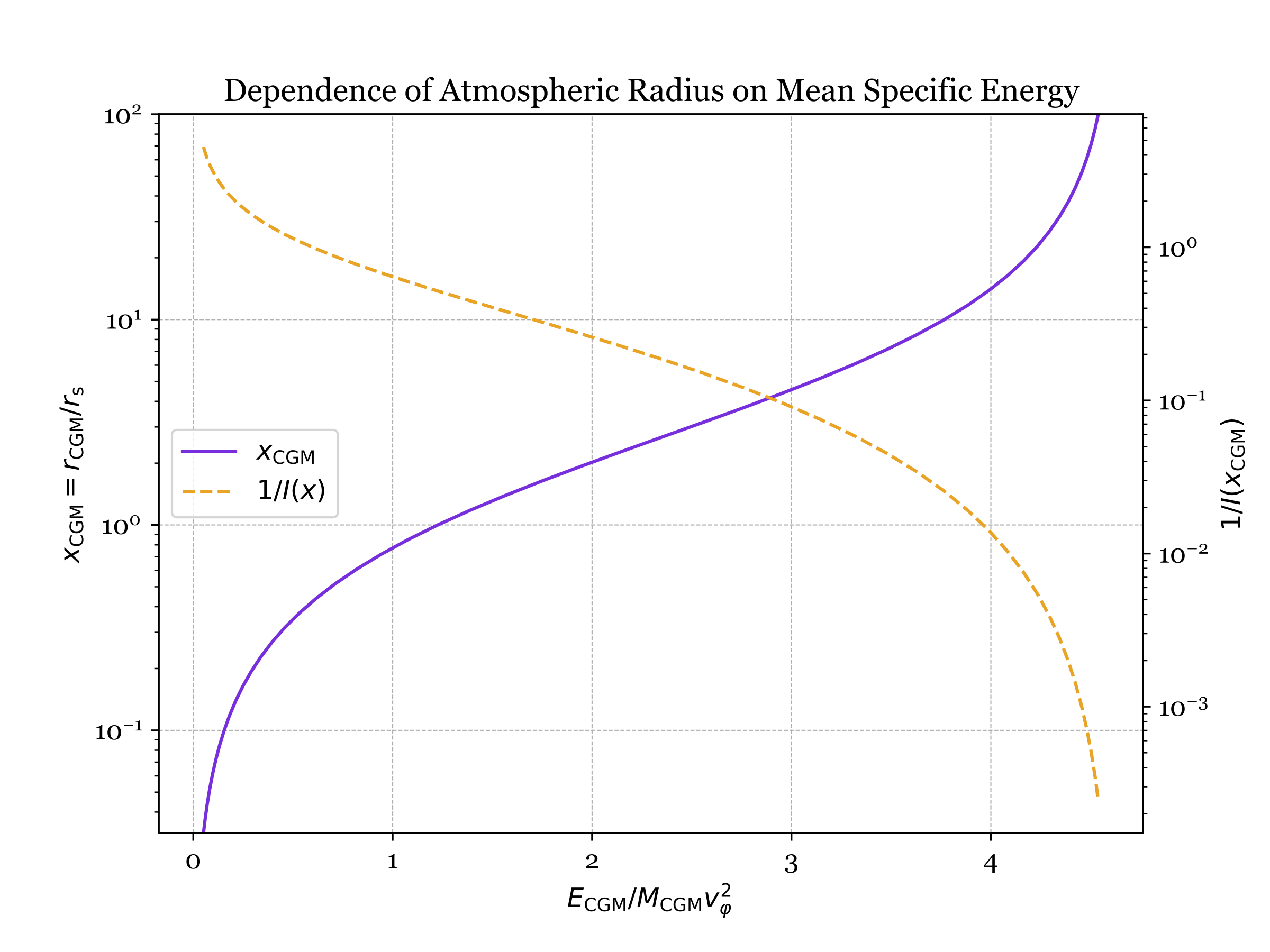
To interpret the plot, consider a halo with a concentration $r_\mathrm{halo} / r_\mathrm{s} = 10$, meaning that $r_\mathrm{halo}$ corresponds to $x = 10$. The solid line shows that the model atmosphere’s mean specific energy within that radius is $\varepsilon_\mathrm{CGM} \approx 3.7 v_\varphi^2$. According to the model, an atmosphere with that specific energy has a radius $r_\mathrm{CGM}$ equal to $r_\mathrm{halo}$, and increasing its specific energy makes $r_\mathrm{CGM}$ larger than $r_\mathrm{halo}$.

Both the solid line and the dashed line show how strongly the model atmosphere’s radius responds to an increase in $\varepsilon_\mathrm{CGM}$. Raising the mean specific energy of an atmosphere with $r_\mathrm{CGM} \approx 10 r_\mathrm{s}$ by an increment similar to $v_\varphi^2$ causes its radius to expand by more than an order of magnitude and lowers its pressure by more than an order of magnitude, because $P_0 \propto 1 / I(x_\mathrm{CGM})$. Note also that the effects of raising $\varepsilon_\mathrm{CGM}$ on atmospheres with $r_\mathrm{CGM} \approx 3 r_\mathrm{s}$ are not as pronounced until they expand beyond $\sim 10 r_\mathrm{s}$.

Adjustable Power-Law Slope

To change the power-law slope of the pressure profile, you can type in a different value of $\alpha$ and execute the plotting code again, or you can use an interactive version of the plotting code with a slider that determines $\alpha$.

This cell defines a function called update_alpha that updates the plot when the slider moves:

def update_alpha(alpha=1.5):
    # To prepare the plot, specify a range of x and determine the range of F(x) and 1/I(x)
    x_values = np.logspace(-1.5, 2, 50)
    y1_values = [F(x,alpha) for x in x_values]
    y2_values = [1/I(x,alpha) for x in x_values]

    # Choose a font
    gfont = {'fontname':'georgia'}
    plt.rcParams['font.family'] = 'georgia' 
    plt.rcParams['font.size'] = 12 

    # Specify a figure size
    fig, ax1 = plt.subplots(figsize=(8, 6))

    # Plot x_CGM as a function of F(x_CGM) using a solid blue-violet line
    ax1.plot(y1_values, x_values, color='blueviolet', label='$x_{\mathrm{CGM}}$')
    ax1.set_xscale('linear')
    ax1.set_yscale('log')
    ax1.set_xlabel(r'$E_\mathrm{CGM} / M_\mathrm{CGM} v_{\varphi}^2$', fontsize=12)
    ax1.set_ylabel(r'$x_\mathrm{CGM} = r_\mathrm{CGM} / r_\mathrm{s}$', fontsize=12)
    ax1.set_ylim(10**-1.5, 10**2)
    ax1.grid(True, linestyle='--', linewidth=0.5)

    # Plot 1/I(x_CGM) as a function of F(x_CGM) using a dashed orange line
    ax2 = ax1.twinx()
    ax2.plot(y1_values, y2_values, color='orange', linestyle='--', label='$1/I(x)$')
    ax2.set_ylabel('$1/I(x_\mathrm{CGM}) \propto P(r_\mathrm{s})$', fontsize=12)
    ax2.set_yscale('log')

    # Add a legend
    lines_1, labels_1 = ax1.get_legend_handles_labels()
    lines_2, labels_2 = ax2.get_legend_handles_labels()
    ax1.legend(lines_1 + lines_2, labels_1 + labels_2, loc='center left')

    # Add a title and show the plot
    plt.title('Dependence of Atmospheric Radius on Mean Specific Energy', **gfont)
    plt.show()

Running the next cell then makes an interactive plot with an adjustable value of $\alpha$:

#   continuous_update=True allows the graph to update while slider is moved
#   continuous_update=False updates the graph after the slider stops moving

alpha_slider = FloatSlider(description=r'$\alpha$', min=1.25, max=2.5, step=0.01, value=1.5,
                           continuous_update=True)
interact(update_alpha, alpha=alpha_slider);

Adjusting the slider shows that increasing $\alpha$ increases the radius of a galactic atmosphere with a given specific energy. The following figure illustrates the relationship between $x_{\rm CGM}$ and $\varepsilon_{\rm CGM} / v_\varphi^2$ for $\alpha = 2$:

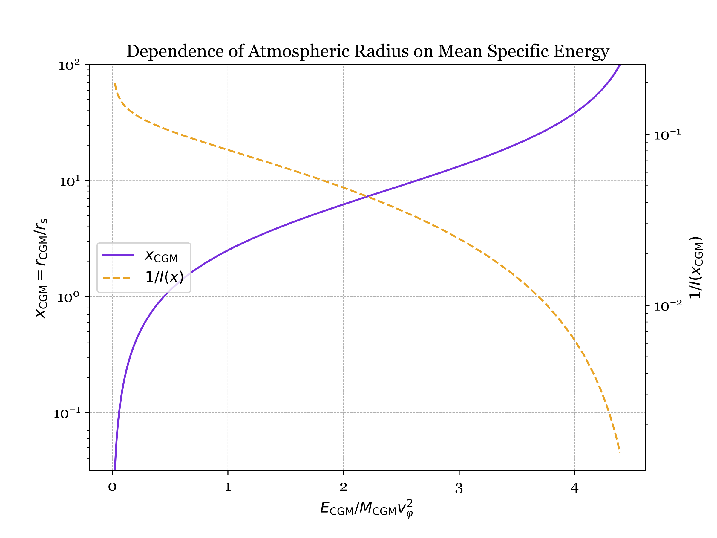
Comparing the two figures on this page shows that increasing $\alpha$ while keeping the atmosphere’s specific energy constant causes its radius to increase. That happens because a hydrostatic atmosphere with a steeper power-law pressure profile (larger $\alpha$) has a lower equilibrium temperature. A greater proportion of its specific energy must be therefore gravitational, meaning that more of the atmosphere’s mass must be at larger radii than in an atmosphere with the same value of $\varepsilon_\mathrm{CGM}$ and a shallower power-law pressure profile.

To go further, see the MSU Generalizable Notebook. As mentioned above, it demonstrates how to implement shape functions that change with radius. It also demonstrates how to implement alternative potential wells, including ones with a central galaxy, and explains how to account for non-thermal atmospheric support energy.